Test for trend in proportions

The test for trends in proportions is also known as the Cochran Armitage test. It performs Chi-squared test for trend in proportions and is used to test whether there is a difference between groups considering the size of the groups. It takes count data from contingency tables where you have one nominal variable with two levels (i.e “Mutated”, “Wild-type”) and the other variable is an ordinal value with minimum 3 values where the variables is naturally ranked
(i.e “Low-exposure” < “Medium-exposure” < “High-exposure”).
The null hypothesis is that there is no trend.

Using data listed in table two we will test if there is a trend over response in patients with breast cancer treated with Olaparib if the tumor has a mutation in a HR gene.
Response is our ordinal value where “CR+PR” represent a tumor shrinkage of 30-100% (Complete or Partial Response), “SD” (Stable disease) represent a shrinkage of less than 30% to 20% increace, while “PD” (Progressive disease) is an increace of more than 20%. Mutational status is our nominal value with the values HR-mutated or Wild-type

First, create a contingency table from vectors.

Wt <- c(8, 10, 3)
HR_mutation <- c(10, 1, 0) 
df = rbind(HR_mutation, Wt)             # Bind vector by rows to a data frame
colnames(df) <- c("CR+PR", "SD", "PD")  # Add response values as column names
df                                      # print data frame

##             CR+PR SD PD
## HR_mutation    10  1  0
## Wt              8 10  3

Count all cases in the table as a sanity check, and summarize the column values with colSums() and save the count as n.

sum(df)               # Total count

## [1] 32

n= colSums(df)        # Count by group/response. Sum column values.
n

## CR+PR    SD    PD 
##    18    11     3

Running the test

Run the test with the base R function:

prop.trend.test(x, n, score = seq_along(x))

With the arguments:

x = Number of events. #Count data, the HR_mutation or Wt vector.

n = Number of trials. #The total number of participants pr ordinal level in trial, the colSum.

score = Group score. #The level and order of the ordinal value. Default value is c(1,2,3, ..etc).
Seq_along(x) as score will assign score = 1, 2, 3 etc to end of vector. Using this function we assume that the data is entered in an ordered fashion from small to large.

prop.trend.test(HR_mutation, n, score = seq_along(HR_mutation))       

## 
## 	Chi-squared Test for Trend in Proportions
## 
## data:  HR_mutation out of n ,
##  using scores: 1 2 3
## X-squared = 7.4455, df = 1, p-value = 0.00636

Either vector from the table will provide the same result, since their proportion will be the same:

prop.trend.test(Wt, n, score = seq_along(Wt))

## 
## 	Chi-squared Test for Trend in Proportions
## 
## data:  Wt out of n ,
##  using scores: 1 2 3
## X-squared = 7.4455, df = 1, p-value = 0.00636

As we can see, the p value is smaller than 0.05, and we can conclude that there is a trend in the proportions of HR-mutated tumors over response.

Summarize categoricals to table

If you have the data in a data frame and need to count the categorical first, you can summarize into a table by the table() function:

# Make a summary table from vectors
Response <- c("CR+PR","CR+PR","CR+PR","CR+PR","CR+PR","CR+PR","CR+PR","CR+PR","CR+PR","CR+PR","CR+PR","CR+PR","CR+PR","CR+PR","CR+PR","CR+PR","CR+PR","CR+PR","SD","SD","SD","SD","SD","SD","SD","SD","SD","SD","SD","PD","PD","PD")
Variable <- c("HR", "Wt", "HR", "Wt", "HR","HR", "HR", "HR", "Wt", "Wt","HR", "Wt", "Wt", "Wt", "HR", "Wt", "HR", "HR", "Wt", "Wt", "Wt", "Wt", "Wt", "Wt", "HR", "Wt", "Wt", "Wt", "Wt", "Wt", "Wt", "Wt")

# Vectors to dataframe, coerse strings to factors, i.e make them "countable"   
Data = data.frame(Variable,Response, stringsAsFactors = TRUE) 
# Specify factor ordering
levels(Data$Response)

## [1] "CR+PR" "PD"    "SD"

# Re-order factor level to correct order:
Data$Response = factor(Data$Response,levels(Data$Response)[c(1,3,2)])
# Check if they are in correct order
levels(Data$Response)

## [1] "CR+PR" "SD"    "PD"

# Make a summary table of the variables you want
MyTable = table(Data$Variable, Data$Response)
MyTable

##     
##      CR+PR SD PD
##   HR    10  1  0
##   Wt     8 10  3

#  Select row by name and unlist().  subset ["ByRow", "ByColumn]
HR_mutation =  unlist(MyTable["HR",])
Wt =       unlist(MyTable["Wt",])
sum(MyTable)

## [1] 32

n= colSums(MyTable)
n

## CR+PR    SD    PD 
##    18    11     3

Onlie calculator

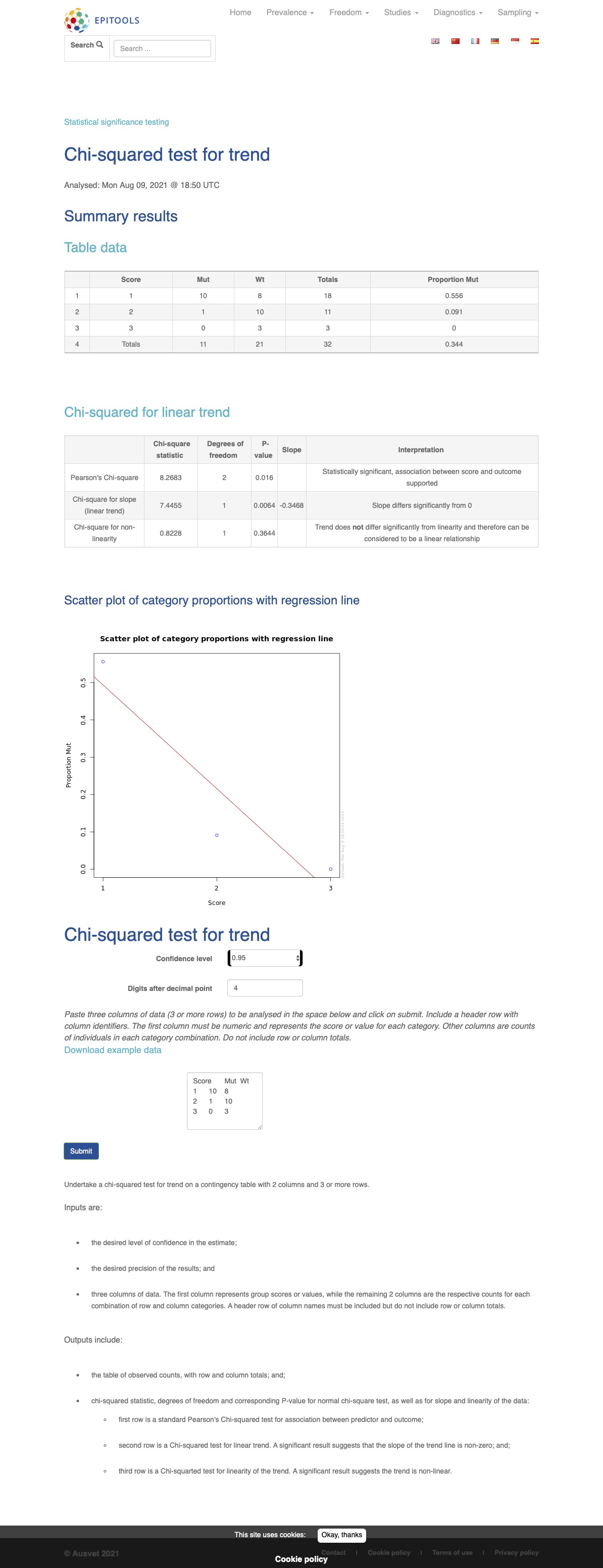
If you want an online calculator solution, epitools has an excellent online calculator here:
https://epitools.ausvet.com.au/trend

A Sample-output of the epitools online calculator for the example above is provided below: